Complexity analysis is very important to building an efficient algorithm. It helps in selecting algorithms and data structures to be used for problems. Lower the time and space complexity more efficient is the algorithm.
Every software engineer should estimate the time and space complexities of the designed solution/program before implementing it. As an inefficient solution can adversely affect the user experience and the cost to use the program/solution.
Since it is impractical to implement and verify the efficiencies of a set of algorithms for a given task, measuring complexities algorithmically is required.
To measure the complexity of an algorithm it is expressed in a form of pseudocode that is mathematically equivalent to the implementation language.
The complexity of an algorithm is given by a function that maps the input size to the number of operations the algorithm will perform to complete the task.
Time Complexity
Time complexity is a function denoting the time taken by an algorithm in terms of the size of the input to the algorithm. Here the term Time does not mean the wall-clock time, it can mean the following:
- Number of memory accesses
- Number of comparisons
- The number of times a statement or a group of statements is executed
For an algorithm wall-clock time is impacted by many factors unrelated to the algorithm itself, such as the computer hardware, OS, libraries, language used, compiler optimization, etc.
Using the time complexity function we can get an independent measure of the algorithm efficiency.
Space Complexity
Space complexity is a function denoting the amount of memory (space) taken by an algorithm in terms of the size of the input to the algorithm. Space complexity includes both spaces used by the input and the auxiliary space. Auxiliary space is the additional space used by the algorithm while executing the statements. For varying size inputs the usual space complexity is O(n) and for fixed input O(1), assuming no quadratic auxiliary space is used. Similar to time complexity notation here also we don’t mean the actual space, but rather an independent unit. A single unit can mean the memory used by a number or string or an object etc.
Notation
For time and space complexity the most common notation used is big O. Big O gives us the asymptotic upper bounds of the complexity. When evaluating it is always preferred to use a meaningful tight upper bound.
For example, the time for bubble sort worst-case complexity is O(n2), but one can also say it as O(n3) this is also an upper bound, but in practice, the correct and meaningful upper bound would be O(n*2).
The lower bound of the complexity is denoted using the notation Omega. The average case of the complexity is denoted using Theta
How to compute time and space complexity
To measure the time complexity of an algorithm we need to count the number of times each operation will occur with respect to the input size of the problem. An input size is an integer number. For example, for a sorting use case length of the array to sort is the input size.
Let’s take the case of merge sort, sorting algorithm
def merge(arr1, arr2):
  # allocate additional space
  temp_arr = []  # O(1)
  i = 0  # O(1)
  j = 0 # O(1)
  while i < len(arr1) and j < len(arr2):  # O(len(arr1) + len(arr2))
    if arr1[i] < arr2[j]:  # O(1)
      temp_arr.append(arr1[I]). O(1)
      i += 1 # O(1)
    else:   # O(1)
      temp_arr.append(arr2[j]). # O(1)
      j += 1 # O(1)
  if i < len(arr1):  # O(len(arr1))
    temp_arr += arr1[i:]. # O(1)
  if j < len(arr2):  # O(len(arr2))
    temp_arr += arr2[j:]  # O(1)
  # space complexity: len(temp_arr)
  return temp_arr # O(1)

N = len(arr1) + len(arr2)
Overall complexity = 3* O(1) + O(n) + 3*O(1) + O(x1) + O(x2) + 3*O(1) ~= O(n)
Space complexity = O(n)

def merge_sort(arr):
  # divide and conquer
  if len(arr) < 2: # O( 1)
    return arr   # O(1)
  mid = len(arr) // 2. # O(1)
  # sort each segments
  arr_1 = merge_sort(arr[0:mid]) # T(n/2)
  arr_2 = merge_sort(arr[mid:])  # T(n/2)
  # merge the two sorted arrays
  return merge(arr_1, arr_2) # O(n)

T(n) = 2*T(n/2) + O(n) + 3 * O(1) = n log(n)
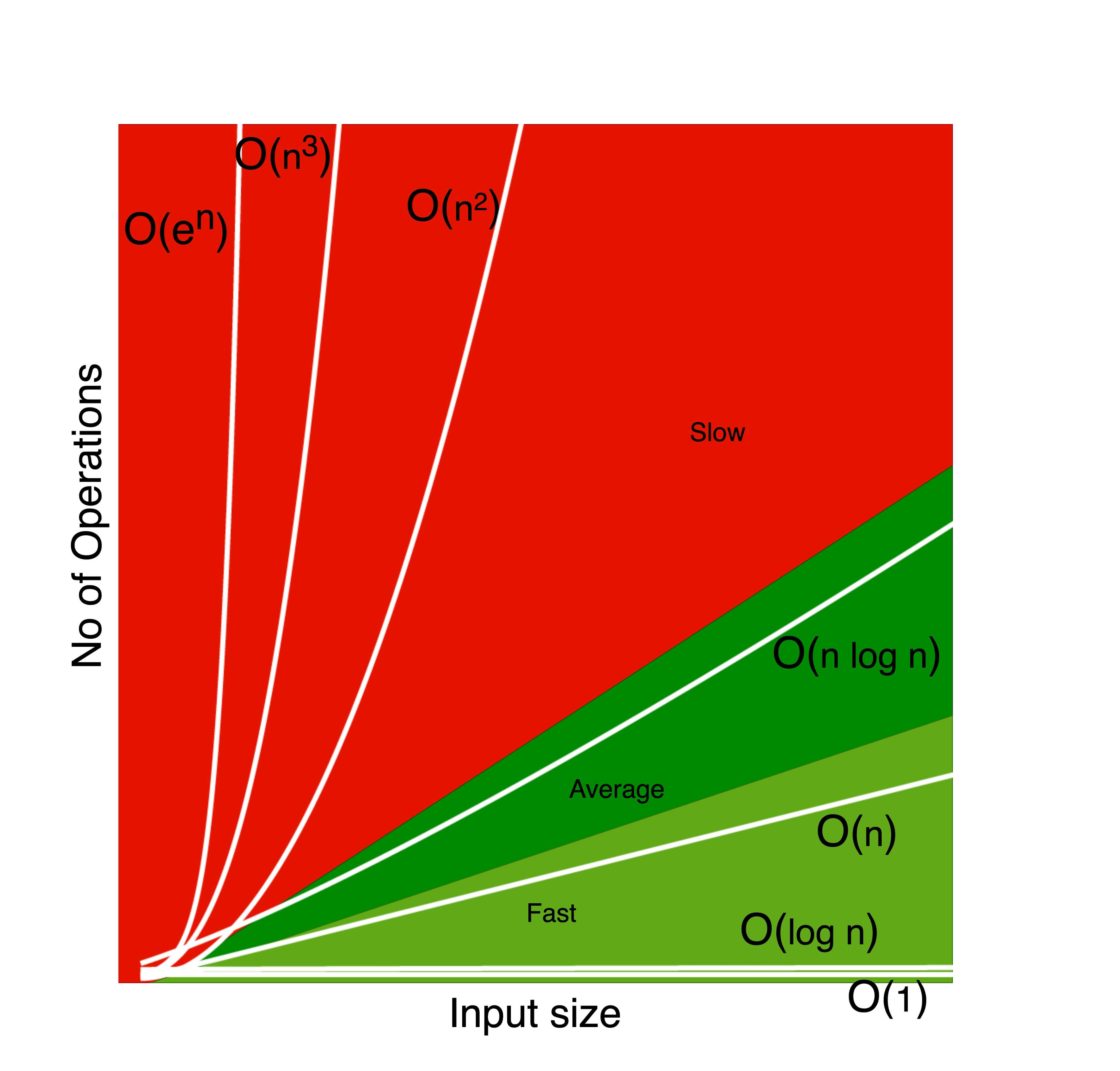
Complexity Plots for common functions
The following diagram shows the variation of complexity with respect to the inout size for some common functions. As we can see that the most efficient functions are O(1) and O(log n), followed by linear O(n).
Most inefficients functions are exponential O(e^n) and polynomials O(n^3) and O(n^2) etc.
A developer should always try to design their algorithm with complexities below O(n log n).
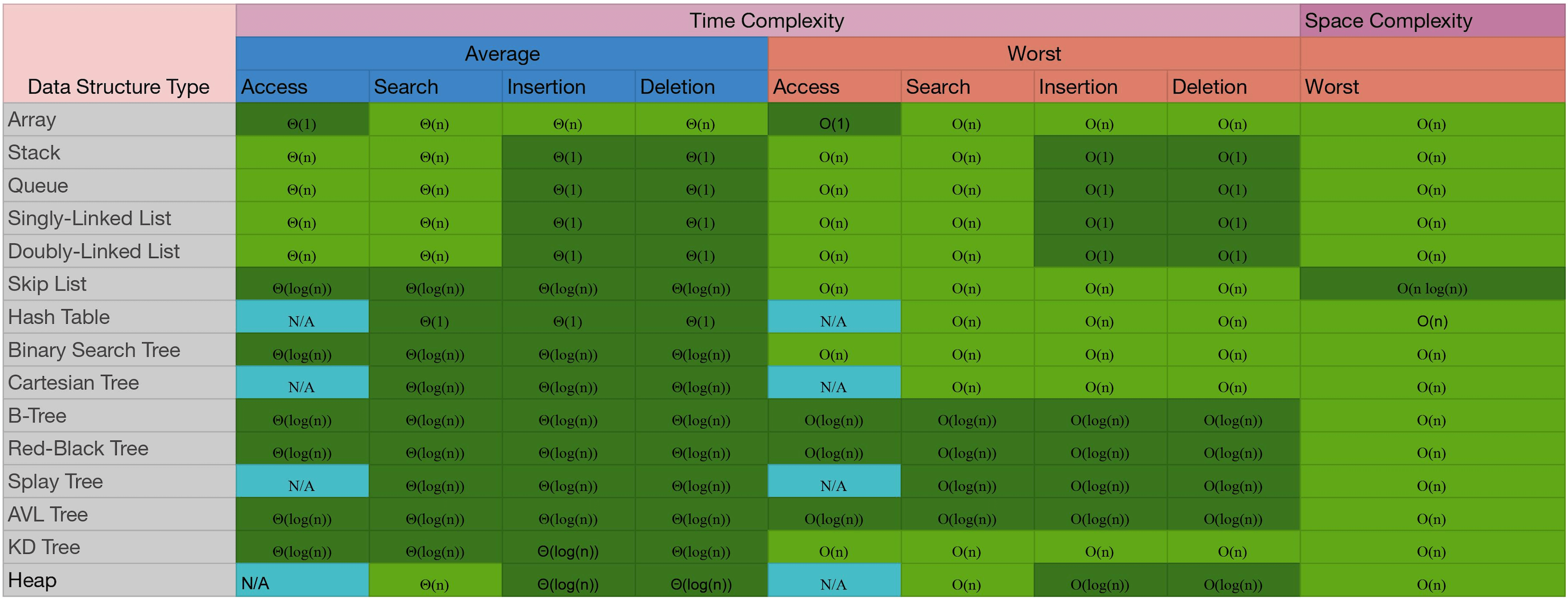
Time and Space complexities of Common Data Structures
Always refer this table before selecting a particular DS for your problem, specifically correlating the problem needs and the complexities of the operations such as search, insert, access and deletion.
For example, for a search dominant problem select hash Table.
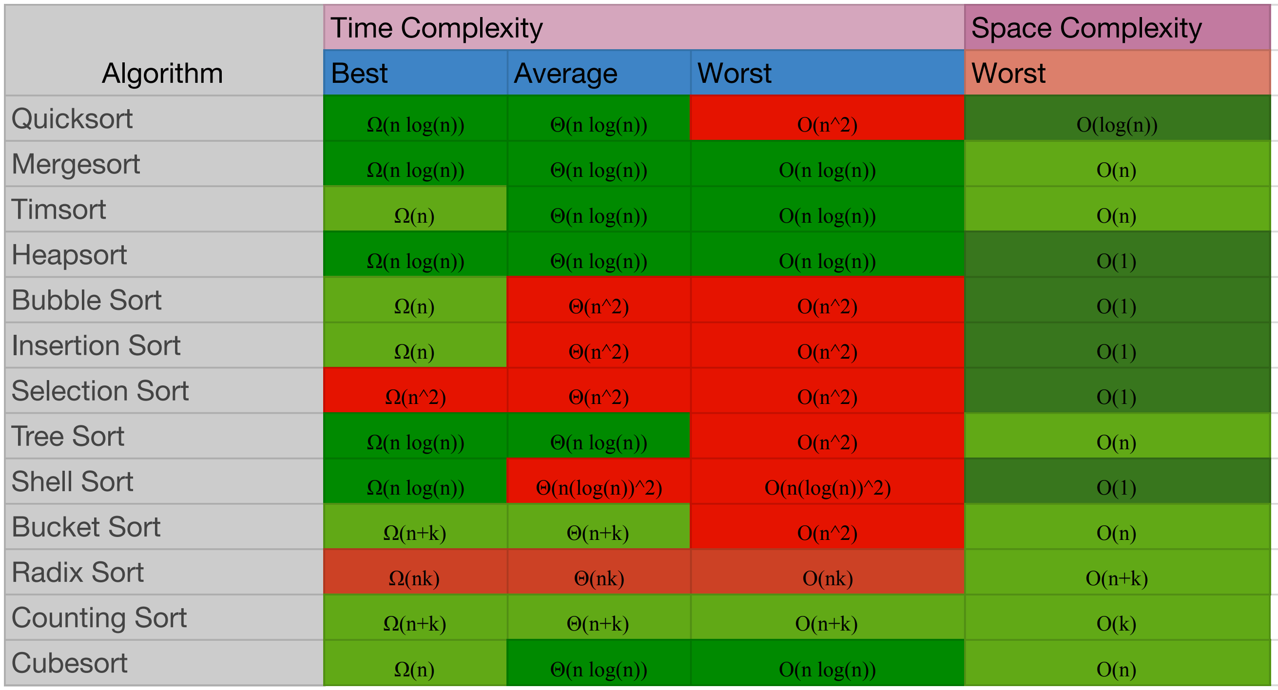
Time and Space complexities of common Sorting algorithms
In practice Quick-sort is always preferred as its implementation does not need too many swaps operation in comparison to Heap-sort and Merge-sort. Swap operations are time consuming. Quick-sort is faster than Heap-sort and Merge-sort.
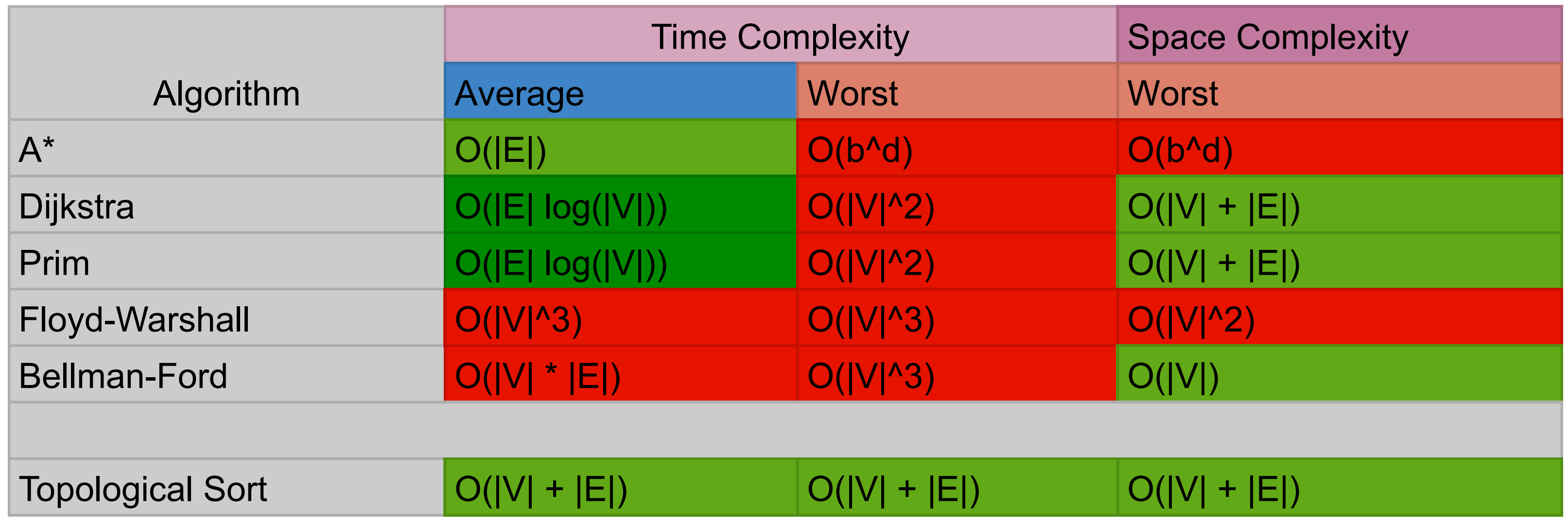
Time and Space complexities of common Graph algorithms
A common application of Graph algorithms is searching shortest path between two nodes in a graph. Such as finding the shortest distance between two places from an available road networks.